ggplot() initializes a ggplot object. It can be used to
declare the input data frame for a graphic and to specify the
set of aesthetic mappings for the plot, intended to be common throughout all
subsequent layers unless specifically overridden.
Value
ggplot
Details
ggplot() is used to construct the initial plot object,
and is almost always followed by a plus sign (+) to add
components to the plot.
There are three common patterns used to invoke ggplot():
ggplot(data = df, mapping = aes(x, y, other aesthetics))ggplot(data = df)ggplot()
The first pattern is recommended if all layers use the same data and the same set of aesthetics, although this method can also be used when adding a layer using data from another data frame.
The second pattern specifies the default data frame to use for the plot, but no aesthetics are defined up front. This is useful when one data frame is used predominantly for the plot, but the aesthetics vary from one layer to another.
The third pattern initializes a skeleton ggplot object, which
is fleshed out as layers are added. This is useful when
multiple data frames are used to produce different layers, as
is often the case in complex graphics.
The data = and mapping = specifications in the arguments are optional
(and are often omitted in practice), so long as the data and the mapping
values are passed into the function in the right order. In the examples
below, however, they are left in place for clarity.
See also
The first steps chapter of the online ggplot2 book.
Examples
example(read10xVisium)
#>
#> rd10xV> dir <- system.file(
#> rd10xV+   file.path("extdata", "10xVisium"),
#> rd10xV+   package = "SpatialExperiment")
#>
#> rd10xV> sample_ids <- c("section1", "section2")
#>
#> rd10xV> samples <- file.path(dir, sample_ids, "outs")
#>
#> rd10xV> list.files(samples[1])
#> [1] "raw_feature_bc_matrix" "spatial"
#>
#> rd10xV> list.files(file.path(samples[1], "spatial"))
#> [1] "scalefactors_json.json"    "tissue_lowres_image.png"
#> [3] "tissue_positions_list.csv"
#>
#> rd10xV> file.path(samples[1], "raw_feature_bc_matrix")
#> [1] "/home/runner/work/_temp/Library/SpatialExperiment/extdata/10xVisium/section1/outs/raw_feature_bc_matrix"
#>
#> rd10xV> (spe <- read10xVisium(samples, sample_ids,
#> rd10xV+   type = "sparse", data = "raw",
#> rd10xV+   images = "lowres", load = FALSE))
#> Warning: 'read10xVisium' is deprecated.
#> Use 'VisiumIO::TENxVisium(List)' instead.
#> See help("Deprecated")
#> # A SpatialExperiment-tibble abstraction: 99 × 7
#> # Features = 50 | Cells = 99 | Assays = counts
#>    .cell              in_tissue array_row array_col sample_id pxl_col_in_fullres
#>    <chr>              <lgl>         <int>     <int> <chr>                  <int>
#>  1 AAACAACGAATAGTTC-1 FALSE             0        16 section1                2312
#>  2 AAACAAGTATCTCCCA-1 TRUE             50       102 section1                8230
#>  3 AAACAATCTACTAGCA-1 TRUE              3        43 section1                4170
#>  4 AAACACCAATAACTGC-1 TRUE             59        19 section1                2519
#>  5 AAACAGAGCGACTCCT-1 TRUE             14        94 section1                7679
#>  6 AAACAGCTTTCAGAAG-1 FALSE            43         9 section1                1831
#>  7 AAACAGGGTCTATATT-1 FALSE            47        13 section1                2106
#>  8 AAACAGTGTTCCTGGG-1 FALSE            73        43 section1                4170
#>  9 AAACATGGTGAGAGGA-1 FALSE            62         0 section1                1212
#> 10 AAACATTTCCCGGATT-1 FALSE            61        97 section1                7886
#> # ℹ 89 more rows
#> # ℹ 1 more variable: pxl_row_in_fullres <int>
#>
#> rd10xV> # base directory 'outs/' from Space Ranger can also be omitted
#> rd10xV> samples2 <- file.path(dir, sample_ids)
#>
#> rd10xV> (spe2 <- read10xVisium(samples2, sample_ids,
#> rd10xV+   type = "sparse", data = "raw",
#> rd10xV+   images = "lowres", load = FALSE))
#> Warning: 'read10xVisium' is deprecated.
#> Use 'VisiumIO::TENxVisium(List)' instead.
#> See help("Deprecated")
#> # A SpatialExperiment-tibble abstraction: 99 × 7
#> # Features = 50 | Cells = 99 | Assays = counts
#>    .cell              in_tissue array_row array_col sample_id pxl_col_in_fullres
#>    <chr>              <lgl>         <int>     <int> <chr>                  <int>
#>  1 AAACAACGAATAGTTC-1 FALSE             0        16 section1                2312
#>  2 AAACAAGTATCTCCCA-1 TRUE             50       102 section1                8230
#>  3 AAACAATCTACTAGCA-1 TRUE              3        43 section1                4170
#>  4 AAACACCAATAACTGC-1 TRUE             59        19 section1                2519
#>  5 AAACAGAGCGACTCCT-1 TRUE             14        94 section1                7679
#>  6 AAACAGCTTTCAGAAG-1 FALSE            43         9 section1                1831
#>  7 AAACAGGGTCTATATT-1 FALSE            47        13 section1                2106
#>  8 AAACAGTGTTCCTGGG-1 FALSE            73        43 section1                4170
#>  9 AAACATGGTGAGAGGA-1 FALSE            62         0 section1                1212
#> 10 AAACATTTCCCGGATT-1 FALSE            61        97 section1                7886
#> # ℹ 89 more rows
#> # ℹ 1 more variable: pxl_row_in_fullres <int>
#>
#> rd10xV> # tabulate number of spots mapped to tissue
#> rd10xV> cd <- colData(spe)
#>
#> rd10xV> table(
#> rd10xV+   in_tissue = cd$in_tissue,
#> rd10xV+   sample_id = cd$sample_id)
#>          sample_id
#> in_tissue section1 section2
#>     FALSE       28       27
#>     TRUE        22       22
#>
#> rd10xV> # view available images
#> rd10xV> imgData(spe)
#> DataFrame with 2 rows and 4 columns
#>     sample_id    image_id   data scaleFactor
#>   <character> <character> <list>   <numeric>
#> 1    section1      lowres   ####   0.0510334
#> 2    section2      lowres   ####   0.0510334
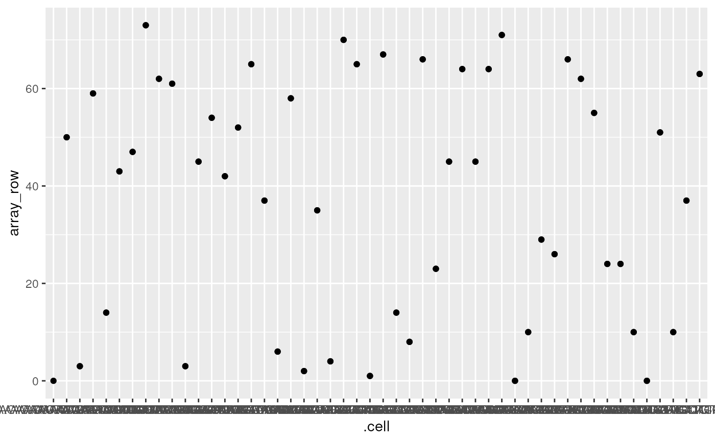
spe |>
    ggplot(ggplot2::aes(x = .cell, y = array_row)) +
    ggplot2::geom_point()
